43 excel pivot table column labels

How to group time by hour in an Excel pivot table? Right-click any time in the Row Labels column, and select Group in the context menu. See screenshot: 5. In the Grouping dialog box, please click to highlight Hours only in the By list box, and click the OK button. See screenshot: Now the time data is grouped by hours in the newly created pivot table. See screenshot: Note: If you need to group time data by days and hours … Excel Pivot values as column labels - Stack Overflow If you have Excel for Office 365 (or Excel 2021) with the FILTER function, you can use the following: Note that I used a table with structured references for the data source. This has advantages in editing the table in the future. For "pivot" header: =TRANSPOSE(SORT(UNIQUE(Table1[Country]))) For the columns:

Change Blank Labels in a Pivot Table - Contextures Blog You can type any text to replace the (Blank) entry, even a space character, but you can't clear the cell and leave it empty: Select one of the Row or Column Labels that contains the text (blank). Type N/A in the cell, and then press the Enter key. Note: All other (Blank) items in that field will change to display the same text, N/A in this ...

Excel pivot table column labels

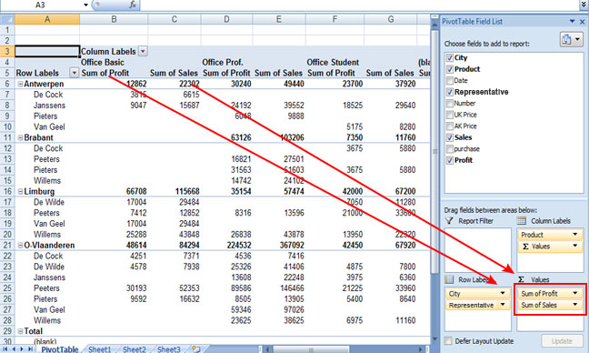
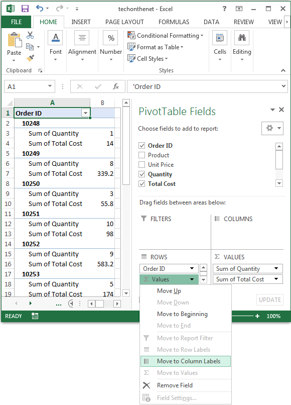
Pivot table row labels side by side - Excel Tutorials You can copy the following table and paste it into your worksheet as Match Destination Formatting. Now, let's create a pivot table ( Insert >> Tables >> Pivot Table) and check all the values in Pivot Table Fields. Fields should look like this. Right-click inside a pivot table and choose PivotTable Options…. Check data as shown on the image below. How to Customize Your Excel Pivot Chart Data Labels - dummies The Data Labels command on the Design tab's Add Chart Element menu in Excel allows you to label data markers with values from your pivot table. When you click the command button, Excel displays a menu with commands corresponding to locations for the data labels: None, Center, Left, Right, Above, and Below. Pivot table - Wikipedia Column labels are used to apply a filter to one or more columns that have to be shown in the pivot table. For instance if the "Salesperson" field is dragged to this area, then the table constructed will have values from the column "Sales Person", i.e. , one will have a number of columns equal to the number of "Salesperson".

Excel pivot table column labels. Excel Pivot Table Group: Step-By-Step Tutorial To Easily Group … Let's start by looking at the… Example Pivot Table And Source Data. This Pivot Tutorial is accompanied by an Excel workbook example. If you want to follow each step of the way and see the results of the processes I explain below, you can get immediate free access to this workbook by subscribing to the Power Spreadsheets Newsletter.. I use the following source data for all … Format column labels in pivot table | MrExcel Message Board Move the field to row labels. Point to the top edge of the field button until the pointer changes to , and then click. Format it and move it back to column labels You must log in or register to reply here. Similar threads VBA to Filter Column Labels of a Pivot Table SanjayGulatiMusafir Nov 25, 2021 Excel Questions Replies 0 Views 204 Nov 25, 2021 Changing Blank Row Labels - Excel Pivot Tables Select one of the Row or Column Labels that contains the text (blank). Type N/A in the cell, and then press the Enter key. Note: All other (Blank) items in that field will change to display the same text, N/A in this example. For more information on pivot tables, see the Pivot Table Topics on my Contextures web site. Excel Pivot Table Subtotals - Contextures Excel Tips Feb 01, 2022 · Creating Pivot Table Subtotals . If your pivot table has only one field in the Row Labels area, you won't see any Row subtotals. In the pivot table shown below, Service is in the Row Labels area, Lead Tech is in the Column Labels area, and Labor Cost is in the Values area.

How to make row labels on same line in pivot table? Make row labels on same line with PivotTable Options You can also go to the PivotTable Options dialog box to set an option to finish this operation. 1. Click any one cell in the pivot table, and right click to choose PivotTable Options, see screenshot: 2. Pivot Table column label from horizontal to vertical Pivot Table column label from horizontal to vertical After pivot table and with grouping, some column labels have been showed but the caption is on the top. What i want is put the column header at the left of the row as vertical red text show as below. However, i cannot do this, it said "We cant change this part of pivot table". Design the layout and format of a PivotTable In the PivotTable, right-click the row or column label or the item in a label, point to Move, and then use one of the commands on the Move menu to move the item to another location. Select the row or column label item that you want to move, and then point to the bottom border of the cell. Remove PivotTable Duplicate Row Labels - Excel Help Forum The best solution here is to filter that field out in the raw data, select a cell which has the issue, copy and paste it across the column. And for the Vendor Name issue, you can use the same solution. Hope this clarifies.. Regards, Chandra Please click on the 'Add Reputation' button at the bottom of my post if I was helpful in resolving the issue.

Hide Excel Pivot Table Buttons and Labels Right-click any cell in the pivot table In the pop-up menu, click PivotTable Options In the PivotTable Options dialog box, click the Display tab To hide all of the expand/collapse buttons in the pivot table: Remove the check mark from the option, Show expand/collapse buttons Pivot Table Banded Columns by Label - MrExcel Message Board Code: Sub PtBandedColByLabel () Dim pt As PivotTable, cr As Range, db As Range, c% Set pt = ActiveSheet.PivotTables (1) Set cr = pt.ColumnRange Set db = pt.DataBodyRange Dim rowCount As Integer rowCount = pt.TableRange1.Rows.Count 'count of all rows in the table Dim rowOffset As Integer ' rowOffset = 2 'cell values Dim prevValue As String Dim ... How to insert a blank column in pivot table? - Chandoo.org 16/04/2015 · We all know pivot table functionality is a powerful & useful feature. But it comes with some quirks. For example, we cant insert a blank row or column inside pivot tables. So today let me share a few ideas on how you can insert a blank column. But first let's try inserting a column Imagine you are looking at a pivot table like above. And you want to insert a column or row. … Automatic Row And Column Pivot Table Labels - How To Excel At Excel Select the data set you want to use for your table The first thing to do is put your cursor somewhere in your data list Select the Insert Tab Hit Pivot Table icon Next select Pivot Table option Select a table or range option Select to put your Table on a New Worksheet or on the current one, for this tutorial select the first option Click Ok

Lesson 55: Pivot Table Column Labels - Swotster

Excel Pivot Table Group: Step-By-Step Tutorial To Group Or ... In fact, as mentioned in Excel 2016 Pivot Table Data Crunching: Each time you create a new pivot table in Excel 2016, Excel automatically shares the pivot cache. Pivot Cache sharing has several benefits. Most notably, as I mention above, it reduces memory requirements and file size vs. the scenario where the Pivot Cache isn't shared.

Excel Pivot Table Report - Sort Data in Row & Column Labels & in Values Area, use Custom Lists

Excel Pivot Table Subtotals - Contextures Excel Tips 01/02/2022 · Creating Pivot Table Subtotals . If your pivot table has only one field in the Row Labels area, you won't see any Row subtotals. In the pivot table shown below, Service is in the Row Labels area, Lead Tech is in the Column Labels area, and …

Excel Pivot Table tutorial – how to make and use PivotTables in Excel

How to Create a Pivot Table in Excel: A Step-by-Step Tutorial Dec 31, 2021 · Every pivot table in Excel starts with a basic Excel table, where all your data is housed. To create this table, simply enter your values into a specific set of rows and columns. Use the topmost row or the topmost column to categorize your values by what they represent.

How to Sort Data in a Pivot Table | Excelchat

Repeat All Item Labels In An Excel Pivot Table - MyExcelOnline You can then select to Repeat All Item Labels which will fill in any gaps and allow you to take the data of the Pivot Table to a new location for further analysis. STEP 1: Click in the Pivot Table and choose PivotTable Tools > Options (Excel 2010) or Design (Excel 2013 & 2016) > Report Layouts > Show in Outline/Tabular Form

Excel: Grouping pivot table entries

Expand Pivot Table Column labels vertically / downwards Expand Pivot Table Column labels vertically / downwards. As we know we can expand/collapse Row Headers or Column Headers in Pivot Tables to reveal details. When we expand column headers, it expands rightwards. My objective is to make it expand downwards (vertically). You can see in the attached images that clicking the plus sign expands a ...

Excel pivot table categorical variables the same in multiple columns (histogram) - Super User

How to Format Excel Pivot Table - Contextures Excel Tips 23/05/2022 · Keep Formatting in Excel Pivot Table. A pivot table is automatically formatted with a default style when you create it, and you can select a different style later, or add your own formatting. For example, in the pivot table shown below, colour has been added to the subtotal rows, and column B is narrow. Formatting Disappears. However, some of that pivot table …

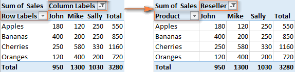
Pivot Table Multiple Row Labels Side By Side

How to Use Excel Pivot Table Label Filters In an Excel pivot table, you might want to hide one or more of the items in a Row field or Column field. To do that, you could click the drop down arrow for the Row or Column Labels, then remove the check mark for items you want to remove. For example, to hide the data for 7-Feb-10, you'd click on the check mark to remove it.

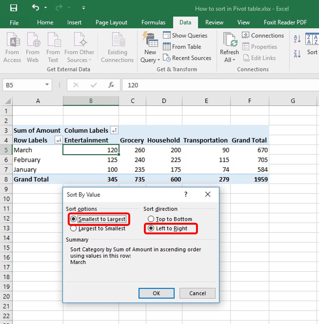
How to Sort Pivot Table | Custom Sort Pivot Table | A-Z, Z-A Order

How to Create a Pivot Table in Excel: A Step-by-Step Tutorial 31/12/2021 · Every pivot table in Excel starts with a basic Excel table, where all your data is housed. To create this table, simply enter your values into a specific set of rows and columns. Use the topmost row or the topmost column to categorize your values by what they represent. For example, to create an Excel table of blog post performance data, you might have a …

How can I fill the empty labels with the headings in a Pivot Table

Pivot table - Wikipedia Column labels are used to apply a filter to one or more columns that have to be shown in the pivot table. For instance if the "Salesperson" field is dragged to this area, then the table constructed will have values from the column "Sales Person", i.e. , one will have a number of columns equal to the number of "Salesperson".

Creating Excel pivot tables ‒ Qlik NPrinting

How to Create Excel Pivot Table [Includes practice file] 15/01/2022 · Using an Excel pivot table, you can organize and group the same data in ways that start to answer actionable questions like: ... There are also ways to filter the data using the controls next to Row Labels or Column labels on the pivot table. You may also drag fields to the Report Filter quadrant. Troubleshooting Excel Pivot Tables . You might encounter several …

MS Excel 2013: Display the fields in the Values Section in multiple columns in a pivot table

How to Add a Column to a Pivot Table - Excel Tutorials Add a Column to a Pivot Table Adding the Data to the Data Model For this example, we will use the table with basketball players from the NBA league, some of their stats, and their salaries. We will select the whole table and then go to the Insert tab and then Pivot Table. A familiar pop-up window will appear:

How to Create a MS Excel Pivot Table – An Introduction | SIMPLE TAX INDIA

Row labels not showing correctly in pivot table - Excel Help Forum Re: Row labels not showing correctly in pivot table. You can't rename a row or column header to a name that is part of the data, but you can easily type in the same name with a leading or trailing space. One spreadsheet to rule them all. One spreadsheet to find them. One spreadsheet to bring them all and at corporate, bind them.

Create a pie chart from distinct values in one column by grouping data in Excel - Super User

Use column labels from an Excel table as the rows in a Pivot Table Highlight your current table, including the headers Then from the Data section of the ribbon, select From Table Highlight all the columns containing data, but not the Year column, and then select Unpivot Columns Close the dialog and keep the changes. Excel should place the unpivoted data into a new worksheet, looking something like this:

vba - Displaying rows based on column label in Excel for a Pivot Table - Stack Overflow

How to Move Excel Pivot Table Labels Quick Tricks To move a pivot table label to a different position in the list, you can use commands in the right-click menu: Right-click on the label that you want to move Click the Move command Click one of the Move subcommands, such as Move [item name] Up The existing labels shift down, and the moved label takes its new position. Type Over Another Label

How to Sort Pivot Table Row Labels, Column Field Labels and Data Values with Excel VBA Macro ...

Combining Column Values in an Excel Pivot Table - Stack Overflow May 14, 2018 · In your pivot table, Select the Pivot Table Tools> Analyze tab, then "Fields, Items",then pull down to"Calculated fields". Enter a name for the generated field, and the formula you want to use: In my example, I added the fields Fruit and Vegi's from my available pivot table fields (which is based on my data table).

How to Sort Pivot Table Row Labels, Column Field Labels and Data Values with Excel VBA Macro ...

Excel tutorial: How to filter a pivot table by rows or columns When you add a field as a row or column label in a pivot table, you automatically get the ability to filter the results in the table by items that appear in that field. Let's take a look. This pivot table is displaying just one field: Total Sales. After we add Product as a row label, notice that a drop-down arrow appears in the header area.

Share :